Abstract
This paper examines to what extent energy efficiency, interpreted as a property-level dimension of climate transition risk, is capitalised into residential sale prices and whether that relationship became more salient during the recent energy shock. Using a linked property-level sample of 5,165,642 housing transactions across 336 England-and-Wales local authorities, matched from HM Land Registry Price Paid data to domestic EPC records through unique property reference number (UPRN) linkage, the paper estimates a hedonic model of log price per square metre with selected structural controls, postcode-sector fixed effects, and sale-quarter fixed effects.
The strongest evidence comes from the baseline EPC specifications. Overall, energy efficiency is priced into this housing sample, but in a distinctly non-linear way: the clearest pattern is a discount for the most inefficient dwellings, especially below band D, rather than a smooth premium ladder across the highest bands. The equivalent continuous EPC-score specification points in the same direction, confirming that better measured energy performance is associated with higher prices on average.
The paper then goes on to test whether an EPC-implied running-cost proxy helps explain that relationship more directly, as a channel. Here the evidence is mixed, as the coefficient is not stable in sign across reasonable sample treatments. A final extension finds that this proxy becomes more negative after October 2021, consistent with energy-related housing attributes becoming a more important consideration to purchasers during the shock period, although this result remains short-run and should be interpreted cautiously. Overall, the findings suggest that energy performance is already reflected in residential prices and forms an economically relevant dimension of housing quality and risk in this sample.
1. Introduction
Climate transition risk has become increasingly significant in the UK residential property market, as energy efficiency influences residential values through expected running costs, vulnerability to future policy tightening, and sensitivity to energy-price shocks. Energy Performance Certificates (EPCs) offer a practical means to quantitatively assess transition risk, as they summarise the energy efficiency of individual dwellings and are directly linked to government regulations and anticipated energy costs. This is relevant for property valuation because energy-inefficient properties are likely to incur higher running costs, face greater exposure to stricter standards, and exhibit heightened price sensitivity during periods of energy market instability. The recent energy crisis accentuated these disparities by increasing the cost of heating inefficient homes and highlighting the importance of household energy exposure (Fuerst et al., 2015; Department of Energy & Climate Change, 2013; Hill et al., 2023).
This study investigates whether climate transition risk is capitalised into residential sale prices at the property level, using EPC information as an indicator of a dwelling’s energy efficiency and exposure to energy-cost pressures. Specifically, it examines whether more energy-efficient properties command higher prices and whether this relationship intensified during the recent energy-price shock (Fuerst et al., 2015; Fuerst et al., 2016; Hill et al., 2023).
The empirical analysis employs a large, linked property-level dataset constructed by matching HM Land Registry transaction data to domestic EPC records using UPRN-based linkage (HM Land Registry, 2025; Ministry of Housing, Communities and Local Government, 2025; University of Bristol Data Centre, 2024). The final estimation sample comprises 5,165,642 transactions across 336 local authorities in England and Wales. A hedonic pricing framework is applied to estimate the relationship between sale prices and energy efficiency, controlling for key structural housing characteristics. The primary focus is on whether energy efficiency is capitalised into prices in the baseline specifications. Additionally, a running-cost proxy is used to investigate the underlying mechanism, and a post-crisis extension tests whether energy-related housing attributes became more salient during the recent energy crisis. The following section presents the conceptual framework and situates this study within the existing literature.
2. Conceptual Framework and Literature
Climate transition risk may affect residential property values because a dwelling's energy efficiency influences both its expected running costs and its exposure to future regulation and energy price increases. In the UK, Energy Performance Certificates (EPCs) provide a practical way to assess this dimension of housing quality at the property level. The basic economic intuition is that buyers should be willing to pay more for properties that are cheaper to run, less exposed to tightening minimum standards, and less vulnerable to future energy price shocks. In this sense, the relevant mechanism is not simply the EPC label itself, but the future financial implications of energy efficiency for the owner. If those future costs and risks matter to buyers, they should be capitalised into transaction prices. This provides the conceptual basis for testing whether energy efficiency is reflected in prices using both discrete EPC bands and a continuous EPC-score measure.
The earlier literature on this topic rarely studied EPC labels directly. Instead, it tended to proxy energy efficiency through energy bills, thermal integrity, or related housing characteristics. Across this earlier work, the broad finding was generally positive. Households appeared willing to pay for dwellings with lower expected energy costs. However, as Laquatra et al. (2002) note, much of this evidence relied on small and highly localised samples, which limited generalisability. These studies were still important because they established the basic proposition that energy efficiency could be valued in housing markets, but they were less well suited to identifying broad market-wide pricing patterns.
Energy labelling grew increasingly common, so the literature subsequently shifted from indirect proxies towards the actual pricing of labels. Evidence from countries with degrees of certificate coverage generally shows the same pattern: more energy-efficient homes tend to sell at premiums, less efficient homes at discounts, and interpretation becomes harder when coverage is incomplete or complicated. The Australian Bureau of Statistics (2008), Brounen and Kok (2011), and Hyland et al. (2013) all report results consistent with this pattern. For the present paper, the most relevant evidence comes from the UK. Fuerst et al. (2015) provide the closest benchmark, showing that the more energy-efficient a dwelling, the higher the premium it sells at, while less efficient dwellings sell at discounts, with the strength of the effect varying across property types. Fuerst et al. (2016) report similar evidence for Wales, while Hill et al. (2023) look closer at the underlying mechanism by linking transaction data to improvements recommended by EPC and associated costs. Looking at both, the UK literature strongly supports capitalisation but also suggests that the size and meaning of the estimated premium vary across the housing stock.
Despite this broad pattern of positive findings, the interpretation of EPC premiums is not straightforward. A central issue is that EPC ratings are strongly correlated with other housing characteristics that also affect price, including age, dwelling type, size, location, and overall quality. Older homes, for example, are often both less energy-efficient and systematically different in other respects. As a result, even hedonic models with strongly defensible controls may struggle to isolate the pricing effect of energy efficiency alone. Related problems arise from unobserved and unquantified improvements, since homes with better EPC ratings may also have been modernised in ways that are not fully captured in the data. There is also a conceptual issue: EPC labels may not perfectly capture the channel buyers care about most, namely expected future running costs. A label is therefore a useful signal, but not necessarily a precise measure of the mechanism through which energy efficiency affects value.
Overall, the literature identifies the clear theme that residential markets appear to place value on energy efficiency, but the size and interpretation of that effect remain contested. This means the literature is no longer simply asking whether an EPC premium exists, but what exactly that premium represents. Against this background, this paper first tests whether energy efficiency is capitalised into transaction prices in baseline EPC specifications, using both band-based and continuous-score measures. It then uses a running-cost-based proxy more cautiously, as a way of investigating whether expected energy-cost exposure helps explain part of that relationship. Finally, because household energy exposure became more salient during the recent energy crisis, the paper considers whether the pricing of energy-related housing attributes became more pronounced in the post-crisis period. These expectations motivate the empirical strategy set out in the next section.
3. Data and Empirical Strategy
3.1 Data and Sample Construction
This study combines three linked administrative data sources at the property level. HM Land Registry Price Paid data for transaction prices and sale dates (HM Land Registry, 2025), the Price Paid to UPRN linker to connect transactions to unique properties (University of Bristol Data Centre, 2024), and domestic EPC certificates for energy performance and related dwelling characteristics (Ministry of Housing, Communities and Local Government, 2025). Transactions are matched from the Price Paid identifier through the linker to a UPRN and then to EPC records. Using UPRNs provides a more reliable property-level match than looser address-based linkage. The sample is constructed using a sale-centred pre-sale matching rule and core cleaning process, with full details of the linkage, restrictions, exclusion rule logic, and intermediate sample counts reported in Appendix A.
The final estimation sample covers sales from 3 August 2007 to 24 January 2022 and contains 5,165,642 transactions across 336 mappable England-and-Wales local authorities. It is a national property-level design, which provides broad geographic coverage and is well suited to testing whether energy efficiency is capitalised into residential prices.
3.2 Variable Construction
The dependent variable is the logarithm of transaction price per square metre (sqm). If Pi denotes sale price and Ai total floor area, the outcome is:
Using natural logarithm standardises values across differently sized dwellings and avoids scale bias across property sizes. Coefficients therefore represent percentage changes in price per sqm, not total price. Floor area nevertheless remains in the model because price per sqm still varies with dwelling size.
The baseline energy-efficiency measure is EPC band. To avoid sparse upper categories, bands A and B are collapsed into a single AB group, producing AB, C, D, E, F and G, with D used as the omitted reference category. A continuous EPC score (0–100) is also retained to check that any pricing gradient is not purely an artefact of band coding.
To explore a possible running-cost channel, the paper also constructs EPC-implied expected energy cost intensity (ECI):
measured in £ per sqm per year, where Hi, Li, Wi are the EPC-reported current heating, lighting, and hot-water costs. Dividing by floor area avoids the measure simply scaling with dwelling size. This is treated as a supplementary proxy for expected running-cost exposure rather than a direct measure of realised bills or savings.
Structural controls Xi include log floor area, property type, tenure, new-build status, and a broad construction-age control. Further detail on the regression specification is provided in Appendix B.
3.3 Empirical Model
The empirical framework is a hedonic price model. For dwelling i, sold in postcode sector s and quarter q, the estimating equation is:
where yisq is log price per sqm, Zi is the energy variable of interest, α is the constant term, γ is the coefficient vector on the control variables, Xi is the vector of structural controls, μs denotes postcode-sector fixed effects, τq denotes sale-quarter fixed effects and εisq is the error term. The coefficients are identified by comparing dwellings sold in the same postcode sector and sale quarter, conditional on the included controls.
All four core models use the same estimation sample, controls, and postcode-sector clustered standard errors. Models 1 and 2 establish the baseline capitalisation relationship between energy efficiency and price, while Models 3 and 4 are used more cautiously to explore a running-cost channel and short post-crisis extension.
Model 1 is the baseline EPC-band specification. Model 2 replaces the band dummies with continuous EPC score. Model 3 replaces the EPC score with the EPC-implied running-cost proxy. Model 4 adds a short post-crisis interaction extension where PostCrisisi = 1 for sales on or after 1 October 2021.
Because quarter fixed effects remain in the model, the crisis extension is interpreted narrowly as a test of whether the pricing of expected running-cost exposure intensified after the onset of the energy shock. Two bounded robustness checks are retained: trimming the top and bottom 1 per cent of both price per sqm and energy cost per sqm and re-estimating the model with a tighter 180-day EPC timing rule.
3.4 Estimation Issues and Limitations
The empirical strategy employed is associational rather than causal. Incorporating structural controls, postcode-sector fixed effects, and sale-quarter fixed effects, the resulting coefficients represent conditional price associations rather than treatment effects. Although each EPC predates the sale, EPC measures are administrative assessments rather than indicators of realised energy use. Consequently, expected energy cost intensity serves as a proxy for running-cost exposure rather than actual energy bills.
The external validity of these findings is limited. Estimates are derived from a large, linked multi-authority sample that is not nationally representative. Evidence related to the energy crisis is restricted, as the post-crisis sample comprises 32,314 observations from after 1 October 2021 through January 2022; thus, the interaction term is interpreted as short-run evidence only. Standard errors are clustered by postcode sector, resulting in 7,988 clusters. Although singleton fixed-effect observations are excluded, cluster sizes remain uneven. Correlation and variance inflation factor (VIF) checks indicate overlap among EPC score, property age, new-build status, and expected energy cost intensity; however, these variables are retained because they capture distinct dimensions. The baseline EPC capitalisation result is considered the most robust evidence, while the proxy and crisis interaction effects are interpreted with greater caution.
The sample uses administrative property level records, does not identify individuals, and is only in aggregate statistical form, so does not pose any privacy issues.
4. Results and Discussion
Our empirical approach is structured to produce a clear hierarchy of evidence. Models 1 and 2 provide the main baseline results; Model 3 offers a more tentative test of the running-cost channel; and Model 4 is a post-October 2021 extension.
4.1 Baseline Results
The central empirical result of the paper is that energy efficiency is priced into this housing sample once structural controls, postcode-sector fixed effects, and sale-quarter fixed effects are included. This seems clear in Model 1 and is generally reinforced by Model 2. Taken together, the two baseline specifications show that the relationship between energy performance and price is not a fragile feature of one coding choice but is qualitatively stable across both the band-based and continuous-score specifications.
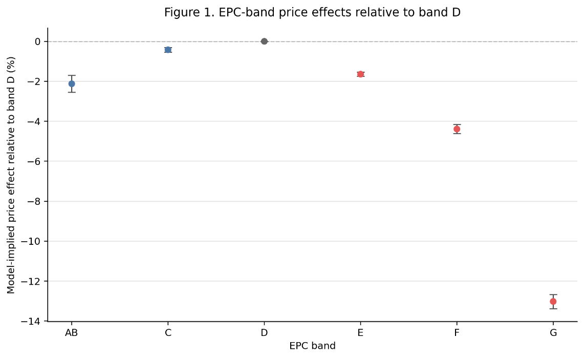
Figure 1: EPC-band price effects relative to band D
Model 1 estimates EPC-band price effects relative to band D. The direct band estimates place AB at -2.1% and band C at -0.4%, while bands E, F, and G fall to -1.6%, -4.4%, and -13.0%, respectively. Band D, therefore, is the local high point. The key takeaway is not that each band delivers a smooth incremental premium, but that the market consistently penalises inefficient homes while behaving much less regularly at the efficient end.
Model 2, the continuous-score specification, points to the same broad conclusion but describes the schedule more simply. It imposes a single slope across the distribution, implying an average price premium of +1.3% per 10 EPC-score points. This matters because it confirms that, on average, better-measured energy performance is associated with higher prices, even though Model 1 shows that this average gradient is not a good description of the entire distribution.
Taken together, the two models point to a distinctly non-linear pattern. The clearest regularity is a strong discount for dwellings below band D, rather than a stable premium ladder among the already-efficient bands. The negative AB and C coefficients should not be read as evidence that buyers penalise energy efficiency at the top of the distribution. Rather, once comparisons are made within postcode sectors and sale quarters, band D appears to operate as the local benchmark, and the coarse AB and C categories do not command an additional premium over it in the flexible specification.
| Model | Baseline Term | Implied Price Effect | 95% CI |
|---|---|---|---|
| Model 1 | EPC band AB vs D | -2.1% | [-2.5%, -1.7%] |
| Model 1 | EPC band C vs D | -0.4% | [-0.5%, -0.3%] |
| Model 1 | EPC band E vs D | -1.6% | [-1.7%, -1.5%] |
| Model 1 | EPC band F vs D | -4.4% | [-4.6%, -4.2%] |
| Model 1 | EPC band G vs D | -13.0% | [-13.4%, -12.7%] |
| Model 2 | EPC score (+10 points) | +1.3% | [+1.2%, +1.4%] |
Table 1: Baseline EPC capitalisation results
4.2 Running-Cost Proxy Results
Model 3 should be interpreted as a channel test rather than as a primary headline result. It examines whether a simple EPC-implied annual running-cost proxy can replicate aspects of the broader baseline pricing pattern. If expected running-cost exposure were the primary mechanism underlying the baseline result, higher expected energy cost intensity would be correlated with lower sale prices.
This expected pattern does not appear consistently. In the full sample, the coefficient for expected energy cost intensity is positive rather than negative, and this positive association persists under the more restrictive 180-day EPC window. The coefficient only becomes negative after excluding extreme values from the sample.
| Variant | ECI Coefficient | Observations | Clusters | R-squared |
|---|---|---|---|---|
| Full sample | 0.0002 (0.0000) | 5,165,642 | 7,988 | 0.8087 |
| Trimmed sample | -0.0008 (0.0001) | 4,966,750 | 7,941 | 0.8026 |
| 180-day EPC window | 0.0002 (0.0000) | 3,580,716 | 7,968 | 0.8113 |
Table 2: Stability of the expected energy cost intensity coefficient
If the EPC-based annual cost proxy were the primary channel through which efficiency is reflected in prices, the coefficient would be expected to remain consistent in direction across these sample treatments. However, this consistency is not observed. The baseline EPC capitalisation result remains valid, but it cannot be attributed solely to a single annual-cost measure. A more plausible explanation is that buyers respond to a broader set of characteristics associated with low efficiency, such as retrofit burden, anticipated inconvenience, potential future policy exposure, and general perceptions of dwelling quality and obsolescence.
4.3 Energy Shock Extension
Model 4 extends the running-cost proxy used in Model 3, but focuses on a more specific question. Instead of examining whether expected running-cost exposure explains prices on average, it investigates whether this exposure became more salient following the onset of the energy shock in October 2021.
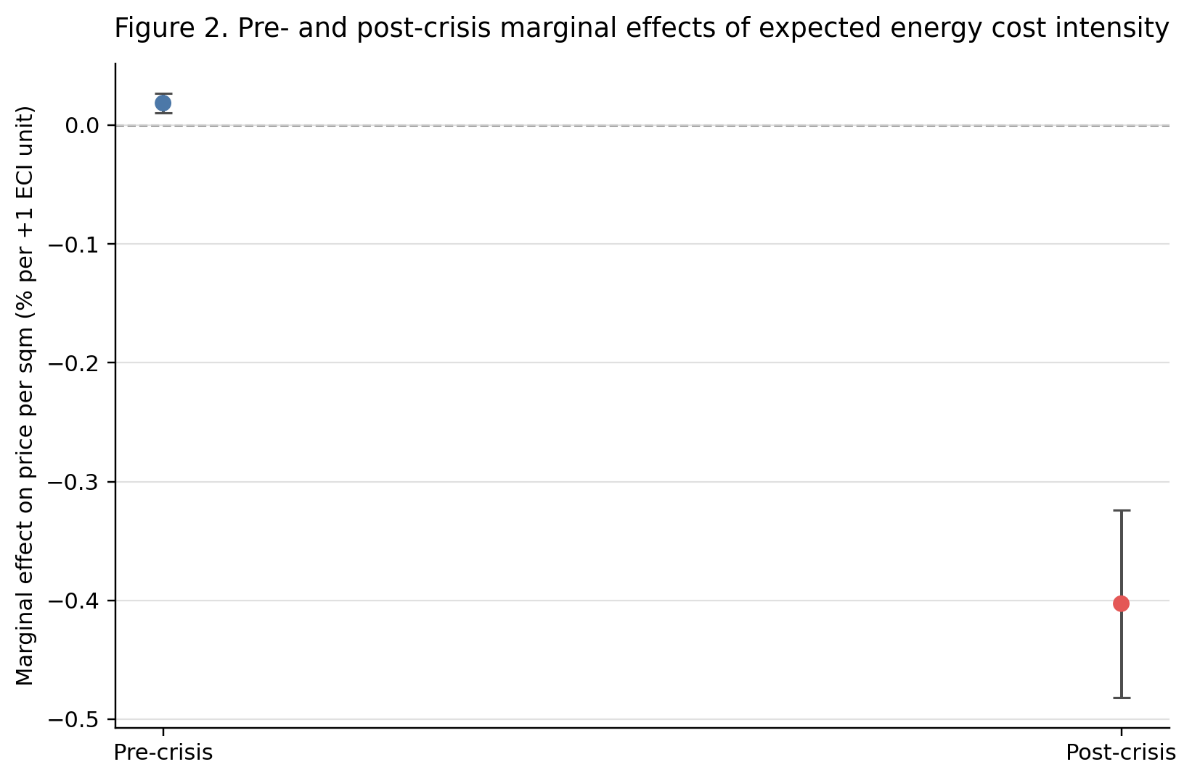
Figure 2: Pre- and post-crisis marginal effects of expected energy cost intensity
Figure 2 illustrates a distinct contrast between the pre-crisis and post-crisis periods. Prior to the energy shock, the marginal effect of expected energy cost intensity is economically negligible. Following the energy shock, the implied marginal effect becomes negative and statistically significant, approximately -0.40%, with a 95% confidence interval of [-0.48%, -0.32%]. This pattern aligns with expectations if running-cost exposure became more salient as energy prices increased sharply.
However, the interpretation of these results should remain more limited than a definitive mechanism finding. Model 4 employs the same EPC-implied running-cost proxy that demonstrated instability in Model 3; therefore, these results should not be interpreted as evidence that annual expected energy costs consistently serve as a stable pricing mechanism. Instead, the findings indicate that the market responded differently to this proxy after the onset of the energy shock. This extension should also be read cautiously because the post-crisis window is short and ends in January 2022.
| Period | Marginal Effect | Approx. Price Effect | 95% CI |
|---|---|---|---|
| Pre-crisis | 0.000185 | 0.018% | [0.011%, 0.027%] |
| Post-crisis | -0.004027 | -0.403% | [-0.482%, -0.324%] |
Table 3: Pre- and post-crisis marginal effects of expected energy cost intensity
5. Conclusion
This study investigated whether energy efficiency, as a property-level dimension of climate transition risk, is capitalised into residential sale prices and whether this relationship intensified during the recent energy shock. The findings indicate that energy efficiency is reflected in sale prices within this housing sample when structural controls, postcode-sector fixed effects, and sale-quarter fixed effects are accounted for.
The most robust evidence is provided by the baseline Energy Performance Certificate (EPC) specifications. Models 1 and 2 collectively demonstrate that the relationship between energy performance and price is not sensitive to a single coding approach. The observed pattern is non-linear: the market imposes greater penalties on inefficient homes than it rewards those with the highest ratings, with the largest discounts occurring below band D. The continuous-score specification supports this finding, indicating that, on average, improved measured energy performance is associated with higher sale prices.
The analysis further explored whether a proxy more closely aligned with expected running-cost exposure could more directly explain the observed pricing pattern. The evidence for this is limited. The EPC-implied energy cost measure does not yield consistent results across reasonable sample treatments, indicating that the baseline capitalisation finding cannot be attributed solely to this annual-cost measure. It is more plausible that buyers respond to a broader set of low-efficiency attributes, such as anticipated running costs, retrofit requirements, potential future policy exposure, and general perceptions of dwelling quality and obsolescence.
A final extension examined whether the salience of this pricing relationship increased following the onset of the energy shock in October 2021. The results support this possibility, as the running-cost proxy appears to have greater significance in the post-crisis period compared to the pre-crisis period. However, this evidence is limited to the short term and should be interpreted with caution. In summary, the results indicate that energy performance represents not only an environmental label but also an economically significant aspect of housing quality and risk. For valuation and policy, the primary implication is that transition-related housing attributes are currently reflected in residential prices within this sample and may become increasingly salient over time.
Appendix A: Cleaning
A.1 Purpose, Scope, and Provenance
This appendix documents the sale-centred cleaning pipeline used to link HM Land Registry Price Paid transactions, the Price Paid to UPRN linker, and domestic EPC certificates and remove observations that were unsuitable for our model. We processed and cleaned property-level data from 336 authorities, resulting in a final cleaned sample of 5,165,661 observations. Before regression estimation, 19 singleton fixed-effect observations are removed, leaving the common estimation sample of 5,165,642 used in the main models.
A.2 Timing-Aware Merge Rule
The linkage process follows the sequence: Price Paid transaction ID, linker, UPRN, and EPC. A retained EPC must correspond to the same UPRN, pre-date the sale, and fall within a 365-day lookback window prior to the transaction date. If multiple certificates meet these criteria, the pipeline selects the closest valid pre-sale certificate, prioritising the latest inspection date and, if necessary, the latest lodgement datetime.
A.3 Sequential Cleaning Losses
| Step | Note | Dropped | Remaining | Retained Share |
|---|---|---|---|---|
| start | PP transactions in authority/date scope | n/a | 15,830,614 | n/a |
| 1 | matched to linker / UPRN | 4,392,878 | 11,437,736 | 72.3% |
| 2 | matched to eligible pre-sale EPC within 365 days | 5,949,722 | 5,488,014 | 48.0% |
| 3 | standard sale filter | 314,126 | 5,173,888 | 94.3% |
| 4 | active record-status filter | 0 | 5,173,888 | 100.0% |
| 5 | valid sale date / postcode / outcode / postcode sector | 1 | 5,173,887 | 100.0% |
| 6 | valid EPC date / band | 5 | 5,173,882 | 100.0% |
| 7 | positive sale price / floor area | 7,842 | 5,166,040 | 99.8% |
| 8 | non-missing heating / lighting / hot-water costs | 9 | 5,166,031 | 100.0% |
| 9 | derived-value validity | 370 | 5,165,661 | 100.0% |
| end | final main-model-ready cleaned sample | n/a | 5,165,661 | n/a |
Table A1: Sample construction and cleaning pipeline
A.4 Final Cleaned Sample Distribution
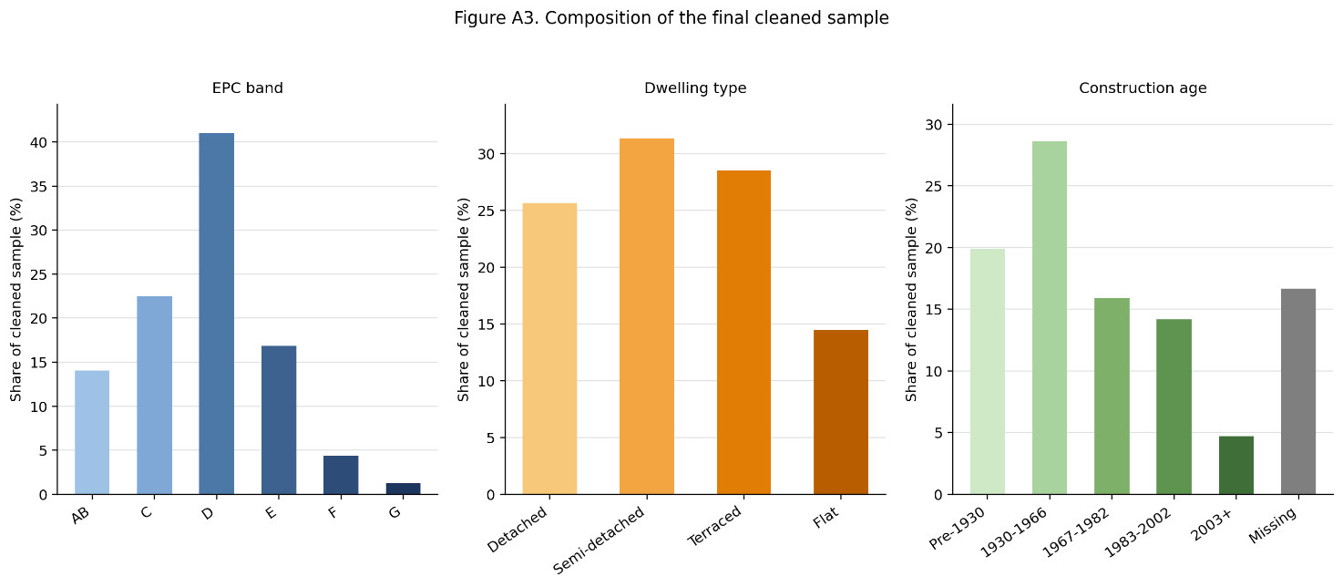
Figure A1: Final cleaned sample distribution across EPC band, dwelling type, and construction age
| EPC Band | Count | Share (%) |
|---|---|---|
| AB | 725,810 | 14.1 |
| C | 1,161,383 | 22.5 |
| D | 2,117,840 | 41.0 |
| E | 871,164 | 16.9 |
| F | 224,847 | 4.4 |
| G | 64,617 | 1.3 |
Table A2: Observation count by band
| Dwelling Type | Count | Share (%) |
|---|---|---|
| Detached | 1,325,068 | 25.7 |
| Semi-detached | 1,619,874 | 31.4 |
| Terraced | 1,473,510 | 28.5 |
| Flat | 747,209 | 14.5 |
Table A3: Observation count by dwelling type
| Construction Age Bin | Count | Share (%) |
|---|---|---|
| Pre-1930 | 1,027,581 | 19.9 |
| 1930–1966 | 1,478,412 | 28.6 |
| 1967–1982 | 822,398 | 15.9 |
| 1983–2002 | 733,055 | 14.2 |
| 2003+ | 243,737 | 4.7 |
| Missing | 860,478 | 16.7 |
Table A4: Observation count by construction age bin
A.5 Derived Variables and Tail Handling
| Metric | Price per square metre | Energy cost per square metre |
|---|---|---|
| Raw min | 4.61 | 0.30 |
| 1st percentile | 659.72 | 3.39 |
| Median | 2,457.63 | 9.54 |
| 99th percentile | 9,821.43 | 26.48 |
| Raw max | 14,100,000.00 | 39,200.00 |
| Winsor lower | 659.72 | 3.39 |
| Winsor upper | 9,821.43 | 26.48 |
Table A5: Statistics and winsorisation thresholds for derived variables
A.6 Timing Distribution and Coverage
The cleaned sample has a median sale-to-EPC gap of 129 days, a mean of 144.8, a 95th percentile of 316, and a hard cap of 365 days.
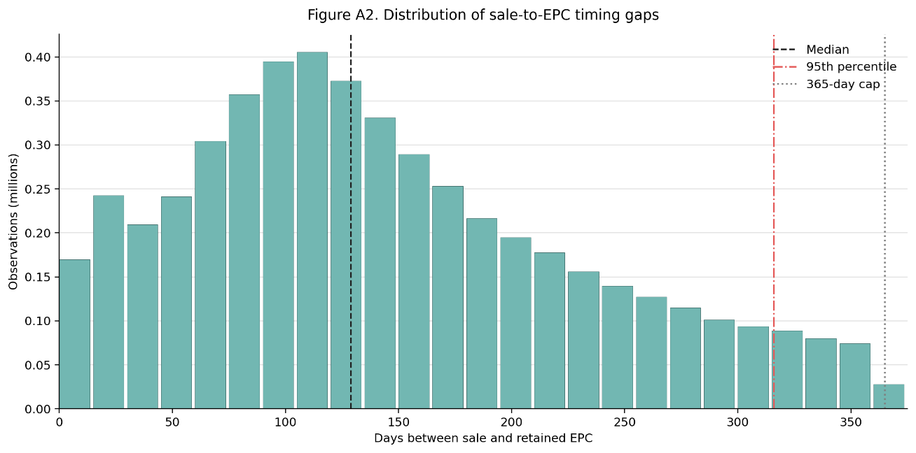
Figure A2: Distribution of days between sale and EPC in cleaned sample
Appendix B: Regression Technical Detail
B.1 Model Design and Common Sample
Appendix B documents and defends the modelling choices made during the empirical phase of the report. All core specifications are estimated on the same sample produced and justified by Appendix A. The comparisons below are about specification design rather than anything to do with sample composition. As before the dependent variable is log transaction price per sqm, and coefficients are therefore interpreted as conditional percentage differences in price per sqm.
| Model | Role | Energy Term | R-squared |
|---|---|---|---|
| Model 1 | Baseline band model | EPC-band dummies, D reference | 0.8097 |
| Model 2 | Band-coding check | Continuous EPC score | 0.8092 |
| Model 3 | Running-cost proxy test | Expected energy cost intensity | 0.8087 |
| Model 4 | Short crisis extension | ECI and ECI × post-crisis | 0.8087 |
Table B1: Core model specification
B.2 Fixed Effects, Clustering, and Inference
Postcode-sector fixed effects are retained to account for sharp variations in house prices across small local markets. Without these controls, persistent local differences could be confounded with both dwelling quality and energy performance. Authority and outcode alternatives are evaluated, but these provide less effective location adjustments compared to postcode-sector fixed effects.
Sale-quarter fixed effects are used to absorb broad temporal shocks, avoiding the need for an additional sale-month fixed-effect parameter. Standard errors are clustered at the postcode sector level to account for the possibility that transactions within the same local market may share unobserved price shocks, neighbourhood valuation effects, and local housing stock characteristics.
B.3 Control Strategy and Supporting Evidence
The structural controls are retained because they address clear confounding risks in this price setting. Floor area is included even though the outcome is price per square metre because unit values still vary systematically with dwelling size. Property type, tenure and new-build status capture major differences in dwelling form and market segment. Construction age bins are included because EPC performance is mechanically related to building vintage, but vintage is also independently valued by buyers.
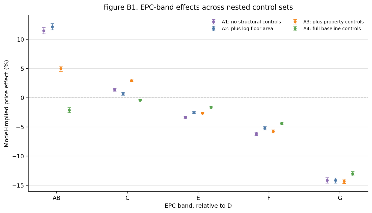
Figure B1: EPC-band percentage effects relative to band D across control sets (95% CI)
| Term | A1: no structural controls | A2: plus log floor area | A3: plus property controls | A4: full baseline controls |
|---|---|---|---|---|
| EPC band AB vs D | +11.5% [+10.9%, +12.0%] | +12.2% [+11.6%, +12.7%] | +5.0% [+4.6%, +5.4%] | -2.1% [-2.5%, -1.7%] |
| EPC band C vs D | +1.4% [+1.1%, +1.6%] | +0.7% [+0.5%, +0.9%] | +2.9% [+2.8%, +3.1%] | -0.4% [-0.5%, -0.3%] |
| EPC band E vs D | -3.4% [-3.5%, -3.2%] | -2.5% [-2.7%, -2.4%] | -2.6% [-2.8%, -2.5%] | -1.6% [-1.7%, -1.5%] |
| EPC band F vs D | -6.2% [-6.5%, -5.9%] | -5.2% [-5.5%, -4.9%] | -5.7% [-6.0%, -5.5%] | -4.4% [-4.6%, -4.2%] |
| EPC band G vs D | -14.1% [-14.6%, -13.7%] | -14.2% [-14.6%, -13.7%] | -14.3% [-14.7%, -13.9%] | -13.0% [-13.4%, -12.7%] |
| R-squared | 0.7437 | 0.7542 | 0.8061 | 0.8097 |
| Within R-squared | 0.0243 | 0.0642 | 0.2618 | 0.2756 |
Table B3: Control results for EPC-band effects
| Candidate Control Test | R² Delta | EPC G Effect | Decision | Reason |
|---|---|---|---|---|
| Authority FE instead of postcode-sector FE | -0.0878 | -13.0% (+0.0 pp vs baseline) | Rejected | Too coarse geographically. Substantially weaker fit than postcode-sector fixed effects. |
| Outcode FE instead of postcode-sector FE | -0.0314 | -12.8% (+0.2 pp vs baseline) | Rejected | Coarser local-market control than postcode sector. Weaker fit and less granular location adjustment. |
| Sale-month FE instead of sale-quarter FE | +0.0001 | -13.0% (+0.0 pp vs baseline) | Not retained | Adds finer time controls but only marginally changes fit and does not change the EPC conclusion. |
| Add EPC-to-sale timing gap | +0.0000 | -13.0% (+0.1 pp vs baseline) | Not retained | Useful as a matching rule, but not a structural valuation control. It barely changes fit or EPC estimates. |
| Add EPC cost components | +0.0009 | -9.2% (+3.8 pp vs baseline) | Rejected | Risks over-controlling the energy-performance channel that the EPC-band model is designed to estimate. |
Table B4: Controls considered but not retained
Appendix C: Regression Results
C.1 Purpose and Reporting Conventions
This appendix reports the detailed regression outputs for the national estimation sample. All reported models include postcode sector fixed effects and sale-quarter fixed effects, but the individual fixed-effect coefficients are omitted from the tables for readability.
| Metric | Value |
|---|---|
| Final common estimation sample | 5,165,642 |
| Authorities | 336 |
| Postcode sectors | 7,988 |
| Sample start date | 2007-08-03 |
| Sample end date | 2022-01-24 |
| Post-crisis observations | 32,314 |
Table C1: Estimation sample summary
| EPC Band | Count | Share (%) |
|---|---|---|
| AB | 725,808 | 14.1 |
| C | 1,161,379 | 22.5 |
| D | 2,117,835 | 41.0 |
| E | 871,158 | 16.9 |
| F | 224,845 | 4.4 |
| G | 64,617 | 1.3 |
Table C2: EPC-band composition
| Variable | Model 1 | Model 2 | Model 3 | Model 4 |
|---|---|---|---|---|
| EPC band AB (vs D) | -0.0215 (0.0022) | |||
| EPC band C (vs D) | -0.0042 (0.0006) | |||
| EPC band E (vs D) | -0.0166 (0.0005) | |||
| EPC band F (vs D) | -0.0449 (0.0012) | |||
| EPC band G (vs D) | -0.1395 (0.0020) | |||
| EPC score | 0.0013 (0.0000) | |||
| Energy cost per sqm | 0.0002 (0.0000) | 0.0002 (0.0000) | ||
| ECI × post-crisis | -0.0042 (0.0004) | |||
| Log floor area | -0.3503 (0.0025) | -0.3514 (0.0025) | -0.3484 (0.0025) | -0.3485 (0.0025) |
| Flat | -0.4343 (0.0040) | -0.4378 (0.0040) | -0.4310 (0.0039) | -0.4310 (0.0039) |
| Semi-detached | -0.1916 (0.0012) | -0.1926 (0.0012) | -0.1892 (0.0012) | -0.1892 (0.0012) |
| Terraced | -0.3300 (0.0018) | -0.3321 (0.0018) | -0.3263 (0.0018) | -0.3264 (0.0018) |
| Leasehold | -0.0641 (0.0031) | -0.0645 (0.0032) | -0.0637 (0.0031) | -0.0637 (0.0031) |
| New build | 0.0764 (0.0024) | 0.0627 (0.0022) | 0.0690 (0.0022) | 0.0691 (0.0022) |
| Observations | 5,165,642 | 5,165,642 | 5,165,642 | 5,165,642 |
| Clusters | 7,988 | 7,988 | 7,988 | 7,988 |
| R-squared | 0.8097 | 0.8092 | 0.8087 | 0.8087 |
| Within R-squared | 0.2756 | 0.2739 | 0.2718 | 0.2718 |
Table C3: Full coefficient estimates for the four core hedonic models
| Variable | Model 3 full | Trimmed | 180-day window |
|---|---|---|---|
| Energy cost per sqm | 0.0002 (0.0000) | -0.0008 (0.0001) | 0.0002 (0.0000) |
| Log floor area | -0.3484 (0.0025) | -0.3268 (0.0021) | -0.3530 (0.0026) |
| Observations | 5,165,642 | 4,966,750 | 3,580,716 |
| Clusters | 7,988 | 7,941 | 7,968 |
| R-squared | 0.8087 | 0.8026 | 0.8113 |
| Within R-squared | 0.2718 | 0.2691 | 0.2752 |
Table C4: Coefficient estimates for bounded robustness checks across alternative samples
References
- Australian Bureau of Statistics (2008) Energy Efficiency Rating and House Price in the ACT: Modelling the Relationship of Energy Efficiency Attributes to House Price. Report for the Department of the Environment, Water, Heritage and the Arts. Canberra: Commonwealth of Australia.
- Brounen, D. and Kok, N. (2011) ‘On the economics of energy labels in the housing market’, Journal of Environmental Economics and Management, 62(2), pp. 166–179. doi:10.1016/j.jeem.2010.11.006
- Ministry of Housing, Communities and Local Government (2025) Energy Performance Certificates for Domestic Buildings.
- Department of Energy & Climate Change (2013) An investigation of the effect of EPC ratings on house prices: final project report. London: Department of Energy & Climate Change.
- Fuerst, F., McAllister, P., Nanda, A. and Wyatt, P. (2015) ‘Does energy efficiency matter to home-buyers? An investigation of EPC ratings and transaction prices in England’, Energy Economics, 48, pp. 145–156. doi:10.1016/j.eneco.2014.12.012
- Fuerst, F., McAllister, P., Nanda, A. and Wyatt, P. (2016) ‘Energy performance ratings and house prices in Wales: an empirical study’, Energy Policy, 92, pp. 20–33. doi:10.1016/j.enpol.2016.01.024
- Hill, R., Pfeifer, N. and Steurer, M. (2023) Energy Efficiency Improvements and Property Values: A Hedonic Analysis of Market Incentives in England and Wales. ESCoE Discussion Paper No. 2023-12. London: Economic Statistics Centre of Excellence.
- HM Land Registry (2025) Price Paid Data.
- Hyland, M., Lyons, R.C. and Lyons, S. (2013) ‘The value of domestic building energy efficiency: evidence from Ireland’, Energy Economics, 40, pp. 943–952. doi:10.1016/j.eneco.2013.07.020
- Laquatra, J., Dacquisto, D.J., Emrath, P. and Laitner, J.A. (2002) ‘Housing market capitalization of energy efficiency revisited’, in Proceedings of the ACEEE Summer Study on Energy Efficiency in Buildings. Washington, DC: American Council for an Energy-Efficient Economy.
- University of Bristol Data Centre (2024) Price Paid Data linked with UPRN.